
Undertaking a PhD project is a great way to start a scientific career, and in many cases a prerequisite for research employment. The number and scope of PhD projects in all scientific disciplines is vast; however the projects themselves are pre-determined by supervisors, and often occur in labs where particular experimental techniques are established and frequently used. Considering time constraints, this is advantageous to the student as there research has direction from the start, and they rapidly acquire the expertise to carry out their research in a particular way and generate data quickly. Success for both student and supervisor. Win-win, surely?
Projects where a student has had to set up research techniques from scratch are more challenging. There can be a great deal more ‘down-time’ while the bugs and inconsistencies are ironed out, but this can provide an opportunity to really consider the research hypothesis and ensure that the particular approach really is the best way to address it. More scientifically satisfying perhaps, especially when the experiments finally start to work, but there’s more of a danger of running out of time, or not generating sufficient data.
Either way, lab work uses increasingly complicated techniques that in many cases have been simplified by technology. There is a danger that lab work can become an exercise in learning to set up and use a particular machine or experimental model, rather than learning underlying principles, adapting the tech to hand, and possibly innovating with alternative approaches to those already established in the lab.
In reality, PhD projects can contain elements of all of the above, and discerning students and supportive supervisors will be aware of the issues. So in order to produce the best scientists who are equipped to approach any research question effectively, there is real value in encouraging PhD students to go back to first principles when addressing the key questions of their research. How does my experimental approach work? Is it the best way to obtain the data needed to test the hypothesis? Are there alternatives? Can I bring something new to the lab? How can I manage the project effectively?
Just one way to support PhD students is by providing or promoting specialized training courses. In the field of electrophysiology for example, there is a superb microelectrode techniques training course which has run annually in September for the last 35 years:
http://www.mba.ac.uk/microelectrode-techniques-cell-physiology
I was able to attend as a PhD student a few (ahem!) years ago, and have had the privilege to help out on the course on seven of the intervening years. This year I was given the opportunity to introduce a new element to the course – high-throughput patch clamp, which gave me the chance to showcase some of the new technologies which are no longer just the preserve of the pharmaceutical industry. The students, as ever, were enthusiastic and keen to experience a variety of electrophysiological recording techniques, right from the first principles of being able to set up a microscope correctly, to fundamental electronics and building their own amplifiers, making sure their solutions have the correct properties for their experiments, and most importantly, knowing that they are using the most appropriate recording technique to capture the signal they want to measure. And as grant-writers and group leaders of the future, they now have an insight into just some of the new technology that is or will be available to them, and may help shape their research direction and ideas about project management.
Courses like this not only provide teaching on research fundamentals and best practice, they are also an invaluable opportunity for knowledge exchange. Every year I learn something new, and it is particularly rewarding to share my own experience with others. So if you are a PhD student or early career researcher, I would encourage you to look for these opportunities (for which it is possible obtain bursaries from organisations to which you may belong as a student member such as the British Pharmacological Society or Physiological Society). And if you are a supervisor or experienced post-doc, please consider supporting these teaching courses by offering your time and experience – everyone will have something to offer, and we are never too old to learn!


Above : The laboratories of the Marine Biological Association in Plymouth (home of the microelectrode techniques course), where Hodgkin and Huxley conducted their Nobel prize-winning research into nerve conduction using the squid giant axon.
Below: main teaching lab.


Blog written by Sarah Lilley.


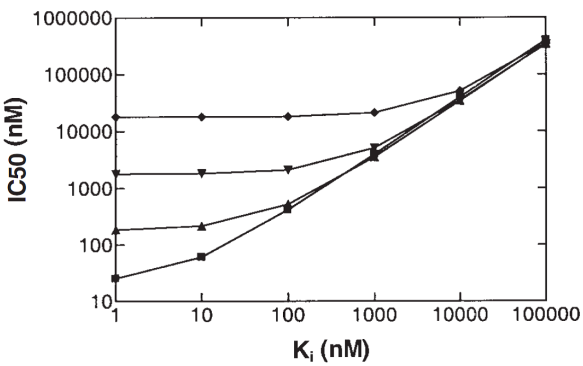


 (Rogers & Aronoff 2016).


